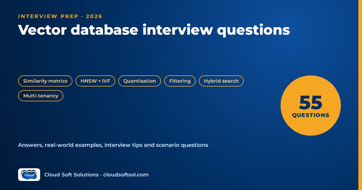
Vector Database Interview Questions and Answers 2026 (55 Questions)

Vector database interview questions in 2026 test whether you understand what happens between "embed the query" and "return the top five chunks": similarity metrics, approximate nearest neighbour indexes such as HNSW and IVF, quantisation, filtering, hybrid search, multi-tenancy and the operational work of keeping an index correct as data changes. This guide collects 55 high-value vector search interview questions with model answers, from fundamentals to index tuning, product trade-offs and production scenarios. The answers are written so you can explain the mechanism, not just name it.

How to use this guide

If you need the concepts first, read vector databases explained and embeddings explained, then come back. What interviewers commonly probe at each level:

• Freshers and junior engineers: what an embedding is, cosine versus dot product versus Euclidean distance, why exact search does not scale and what "approximate" means.
• Mid-level engineers: HNSW and IVF parameters, quantisation, metadata filtering, hybrid search with BM25, and how to measure recall@k.
• Senior and architect roles: multi-tenancy, reindexing without downtime, sharding, cost, choosing between pgvector, a search engine and a dedicated vector database, and structured diagnosis of retrieval incidents.

Questions are numbered continuously. Try answering aloud before reading each model answer, and practise the scenario section with someone playing the interviewer who keeps asking "how would you know?".

• Fundamentals: vectors and similarity (Q1–Q6)
• Embeddings (Q7–Q11)
• ANN index types: HNSW, IVF, PQ, DiskANN (Q12–Q19)
• Recall, latency and memory trade-offs (Q20–Q22)
• Filtering (Q23–Q26)
• Hybrid search and fusion (Q27–Q29)
• Multi-tenancy (Q30–Q31)
• Updates, deletes and reindexing (Q32–Q34)
• Scaling: sharding and replication (Q35–Q36)
• Vector database options compared (Q37–Q39)
• Evaluation and recall@k (Q40–Q42)
• Cost (Q43–Q44)
• Real-world scenario questions (Q45–Q55)
• Key takeaways
• Interview preparation checklist
• FAQ

Fundamentals: vectors and similarity

1. What is a vector database, and what problem does it solve?

Answer: A vector database stores high-dimensional vectors (usually embeddings) alongside an ID and metadata, and answers "which stored vectors are closest to this query vector?" quickly, typically with an approximate nearest neighbour (ANN) index. The problem it solves is similarity search at scale: comparing a query against millions of vectors one by one is too slow for interactive use, so the database builds an index that inspects only a small fraction of candidates. A production vector store also has to do the database work around that: filtering on metadata, inserts, updates and deletes, persistence, replication, access control and backups.

Interview tip: Separate the index algorithm (HNSW, IVF) from the database (storage, filtering, durability, operations). Strong candidates show they know both halves matter.

2. Explain cosine similarity, dot product and Euclidean (L2) distance. When does each fit?

Answer: Cosine similarity measures the angle between two vectors and ignores their length. Dot product (inner product) is the sum of element-wise products, so it grows with both angle alignment and magnitude. Euclidean (L2) distance is the straight-line distance between the two points. Use the metric the embedding model was trained for, which its documentation states. Most text embedding models are trained with a cosine-style objective, so cosine (or dot product on normalised vectors) is typical. Dot product fits when magnitude carries meaning, for example some recommendation models where a larger norm encodes popularity or confidence. L2 is common for image and classical feature vectors and is what many index libraries default to.

Metric	Sensitive to length?	Typical fit
Cosine	No	Text embeddings, semantic search
Dot product	Yes	Normalised text embeddings (fast), recommendation models where norm matters
L2 (Euclidean)	Yes	Image and feature vectors, models trained with L2

3. If vectors are normalised, why do cosine, dot product and L2 give the same ranking?

Answer: For unit-length vectors, the dot product equals the cosine of the angle, and the squared L2 distance equals 2 minus twice the dot product. Because L2 is a monotonic function of the dot product, sorting by smallest L2 distance gives the same order as sorting by largest dot product or largest cosine. That is why many systems normalise embeddings at ingestion and then use the cheaper inner product. One practical trap: the scores differ even when the order does not, so a relevance threshold tuned on cosine scores cannot be copied to an L2 index.

Real-world example: In pgvector, <=> is cosine distance, <#> is negative inner product and <-> is L2. The index must be built with the matching operator class (for example vector_cosine_ops), or the query will not use it.

4. What is the difference between exact k-NN and approximate nearest neighbour search?

Answer: Exact k-NN (brute force or "flat" search) compares the query with every vector and always returns the true top k. Its cost grows linearly with the number of vectors and dimensions. ANN search uses an index structure (graph, clusters, compressed codes) to examine a small subset and returns results that are usually, but not always, the true nearest neighbours. You trade a small, measurable loss in recall for large gains in latency and throughput. The quality of that trade is what "recall@k against exact search" measures.

Interview tip: Say that exact search is still useful: as ground truth for evaluating an ANN index, and for small or heavily filtered candidate sets where scanning is cheaper than walking an index.

5. What is the difference between a vector library like FAISS and a vector database?

Answer: FAISS is a library from Meta for efficient similarity search and clustering of dense vectors. It gives you index types (flat, IVF, PQ, HNSW and combinations, with GPU support for some), but it runs inside your process. Persistence, metadata filtering, concurrent writes, replication, access control and an API are your problem. A vector database wraps an index (sometimes FAISS itself, or its own implementation) in a service that handles those concerns. Libraries fit offline batch jobs, research and embedded use; databases fit shared, continuously updated production workloads.

6. When do you not need a dedicated vector database?

Answer: Often. If your corpus is modest, you already run PostgreSQL, and you need joins with relational data, transactions and existing backups, pgvector inside Postgres is usually the simplest choice. If you already run OpenSearch or Elasticsearch for keyword search, their vector support gives you hybrid search in one system. For a few thousand vectors, an in-memory flat search may be enough. A dedicated vector database earns its place when scale, write rates, filtering performance, multi-tenancy features or operational isolation exceed what your existing stores handle well. The decision is about operational fit, not novelty.

Real-world example: Consider an insurer's internal policy assistant with tens of thousands of chunks and strict audit requirements. Adding a pgvector column to the existing Postgres estate reuses its encryption, backup and access controls; our pgvector RAG tutorial walks through exactly that pattern.

Embeddings

7. How would you choose an embedding model for a vector search system?

Answer: Choose by measured retrieval quality on your own data, then by constraints. Build a small labelled set of real queries with known relevant documents, and compare candidate models on recall@k and MRR. Then weigh language coverage (Indian enterprises often need English plus Hindi, Telugu or Tamil, and mixed-script queries), domain vocabulary, maximum input length versus your chunk size, dimensions (which drive storage and memory), latency, cost per token, and deployment constraints such as data residency or whether the model must run inside your VPC. Public leaderboards are a shortlist, not a decision.

Interview tip: Mention that you would pin the model version and record it with every vector, because changing models later forces a full re-embed (see Q47).

8. How do embedding dimensions affect a vector database?

Answer: Dimensions multiply everything: raw storage is roughly vectors times dimensions times bytes per value, distance computations cost more per comparison, and graph indexes need more memory to stay fast. Higher dimensions can capture more nuance but show diminishing returns. Some models are trained so that a prefix of the vector is itself a usable embedding (often called Matryoshka representation learning), which lets you store shorter vectors and accept a small quality loss. Engines also cap indexable dimensions; for example pgvector's HNSW and IVFFlat indexes support up to 2,000 dimensions for vector and 4,000 for halfvec. Check those limits before choosing a model.

9. Why must queries and documents be embedded with the same model, and what are asymmetric embeddings?

Answer: Each model defines its own vector space. A vector from model A compared with a vector from model B is meaningless, even if the dimensions match, because the coordinates mean different things. Asymmetric retrieval models expect queries and passages to be treated differently, for example with a "query:" versus "passage:" prefix, a task-type parameter, or separate query and document encoders. Short questions and long passages look different, and the model is trained to bridge that gap. Forgetting the query prefix, or using the document mode for queries, quietly reduces recall without any error.

10. What is the difference between dense and sparse vectors?

Answer: Dense vectors have a few hundred to a few thousand dimensions, nearly all non-zero, and capture semantic meaning. Sparse vectors have a dimension per vocabulary term (very large), with only a handful of non-zero weights; BM25 term weights and learned sparse models such as SPLADE produce them. Sparse vectors are strong at exact terms, rare words, product codes and names; dense vectors are strong at paraphrase and intent. Several engines (for example pgvector's sparsevec type, OpenSearch, Elasticsearch, Qdrant, Pinecone, Milvus, Weaviate) support sparse representations or keyword search alongside dense vectors, which is the basis of hybrid search.

11. How does chunking interact with embeddings and the vector store?

Answer: One chunk usually becomes one vector, so chunking decides what the index can find. Chunks that are too large blend several topics into one averaged vector and dilute similarity; chunks that are too small lose context and multiply the vector count, which raises cost and memory. Chunks longer than the model's input limit are silently truncated by some APIs. Store the chunk's parent document ID, position, section heading and access metadata with every vector so you can filter, deduplicate and expand context later. Our guide to RAG chunking strategies covers the options in depth.

ANN index types: HNSW, IVF, PQ and DiskANN

12. How does HNSW work?

Answer: HNSW (Hierarchical Navigable Small World) builds a multi-layer proximity graph. Every vector is a node in the bottom layer, and each node is also placed on higher layers with exponentially decreasing probability, so upper layers are sparse "express lanes". A search starts at an entry point on the top layer, greedily moves to the neighbour closest to the query, and drops down a layer when it cannot improve. On the bottom layer it runs a greedy beam search that keeps a candidate list of size ef_search, and returns the closest k from that list. Inserts follow the same descent and then connect the new node to its nearest neighbours on each layer it belongs to.

Layer 2:  E -------------------- o
          |
Layer 1:  E ------ o ------ o -- o
          |        |
Layer 0:  E-o-o-o--o-o-o-o--o-o-Q*
  greedy descent, then wide search
  at layer 0 with ef_search

Interview tip: Mention that HNSW is fast with high recall but memory-hungry, because it keeps vectors and neighbour lists in memory for good performance, and that deletes are awkward in graphs (Q32).

13. Explain the HNSW parameters M, ef_construction and ef_search.

Answer: M is the maximum number of neighbour connections per node per layer (many implementations allow double that on the bottom layer). Higher M improves recall, especially for high-dimensional data, but increases memory and build time. ef_construction is the size of the candidate list used while inserting; higher values find better neighbours and produce a higher-quality graph at the cost of slower builds. ef_search (called ef or hnsw.ef_search in some systems) is the candidate list size at query time; raising it increases recall and latency, and it should be at least k. M and ef_construction are fixed when the index is built; ef_search can be changed per query or session. As a reference point, pgvector defaults to M 16, ef_construction 64 and ef_search 40.

Parameter	When set	Raising it
M	Build time	Better recall, more memory, slower build
ef_construction	Build time	Better graph quality, slower build
ef_search	Query time	Better recall, higher latency

14. How does an IVF index work, and what are lists and probes?

Answer: IVF (inverted file) clusters the vectors with k-means into a number of lists (also called nlist or partitions), each with a centroid. Every vector is assigned to its nearest centroid's list. At query time the engine finds the closest centroids and scans only those lists; the number scanned is probes (nprobe). More lists make each list smaller and queries faster, but raise the chance that a true neighbour sits in a list you did not probe; more probes recover recall at the cost of latency. Because centroids are learned from data, an IVF index should be built after representative data is loaded and rebuilt if the distribution drifts. pgvector's documentation suggests starting around rows divided by 1,000 lists for up to a million rows, and probes around the square root of lists, then tuning by measurement.

15. What is product quantisation (PQ)?

Answer: Product quantisation compresses vectors by splitting each one into m sub-vectors and replacing each sub-vector with the ID of its nearest centroid from a small codebook learned for that sub-space (commonly 256 centroids, so one byte per sub-vector). A vector of many float32 values becomes m bytes. Distances are approximated with precomputed lookup tables between the query's sub-vectors and the codebook centroids, which is fast. The cost is accuracy: PQ distances are approximate, so systems often retrieve extra candidates and re-rank them with full-precision vectors. PQ is frequently combined with IVF (IVF-PQ) in FAISS and Milvus for very large collections.

16. What are scalar and binary quantisation, and why is rescoring important?

Answer: Scalar quantisation maps each float32 component to a smaller type, such as int8 or float16, reducing memory by a factor of two to four with modest recall loss. Binary quantisation keeps only the sign of each component, one bit per dimension, and compares vectors with Hamming distance; it is a large compression but loses more information, and works better for some models than others. In both cases the standard pattern is oversample and rescore: retrieve several times k candidates from the compressed index, then re-rank them using the original full-precision vectors (kept on disk or in a separate column). pgvector supports this with halfvec, bit and an expression index on binary_quantize(); most dedicated engines expose quantisation as an index option.

17. What is DiskANN, at a high level?

Answer: DiskANN is a family of graph-based ANN methods from Microsoft Research designed for datasets larger than RAM. It builds a graph (called Vamana) that is searched in few hops, stores the full vectors and graph on SSD, and keeps only compressed (PQ) vectors in memory to steer the search. During a query it navigates using the compressed vectors, reads a small number of graph nodes and full vectors from SSD, and re-ranks with full precision. The idea is to serve very large indexes with far less memory than an in-memory HNSW, accepting some SSD latency. Implementations or variants appear in several systems, for example a DiskANN index type in Milvus; check your engine's documentation for what it actually ships.

18. How do you choose between flat, HNSW, IVF and quantised indexes?

Answer: Start from data size, update pattern, memory budget and recall target.

• Flat: small collections, ground truth for evaluation, or tiny filtered subsets. Perfect recall, linear cost.
• HNSW: the default for interactive search when the index fits in memory. High recall at low latency, handles incremental inserts well, costs memory.
• IVF: faster builds and lower memory than HNSW, good for large, relatively static data; recall depends on probes and needs retraining as data drifts.
• IVF-PQ, scalar or binary quantisation: when memory cost dominates; plan for rescoring.
• Disk-based graphs (DiskANN-style): very large collections where RAM is the constraint.

Interview tip: Say you would benchmark two candidates on a sample of your own vectors and queries, measuring recall@k against exact search, p95 latency and memory, rather than choosing from a blog post.

19. What should you know about indexes in pgvector specifically?

Answer: pgvector offers HNSW and IVFFlat. HNSW gives a better speed-recall trade-off, can be created on an empty table and handles inserts well, but builds more slowly and uses more memory; build time improves greatly when maintenance_work_mem is large enough to hold the graph. IVFFlat builds faster and uses less memory but should be created after the table has data, because its lists come from that data. Both are approximate, so a query with a WHERE clause filters after the index scan (Q25). Each index serves one distance operator, and the query must use ORDER BY embedding <op> query LIMIT k for the planner to choose it. Use EXPLAIN ANALYZE to confirm, and CREATE INDEX CONCURRENTLY on a live table.

Recall, latency and memory trade-offs

20. Explain the trade-off between recall, latency and memory in vector search.

Answer: You can usually optimise two of the three. More recall means examining more candidates (higher ef_search or probes), which costs latency, or storing richer structures (higher M, less compression), which costs memory. Lower memory through quantisation or disk-based indexes costs recall or adds latency for rescoring and SSD reads. Lower latency through smaller search parameters costs recall. Build time and write throughput are a fourth axis: higher ef_construction and M slow ingestion. The right point is set by the product: a legal research tool that must not miss a precedent tolerates more latency than an autocomplete box.

Interview tip: Frame it as "recall at a latency budget at a memory cost" and draw the curve: recall rises steeply with ef_search at first, then flattens, while latency keeps climbing.

21. How would you estimate memory for an HNSW index?

Answer: Add the raw vectors and the graph. Raw vectors are number of vectors times dimensions times bytes per value: one million 1,024-dimensional float32 vectors is about 4 GB; at float16 about 2 GB; as binary one bit per dimension, about 128 MB. The graph adds neighbour lists, roughly proportional to M per node (more on the bottom layer) times the size of a node ID, plus per-node overhead. Then add metadata, payload indexes, replicas and headroom for rebuilds and growth. The arithmetic is illustrative; always confirm with the engine's own sizing guidance and a load test, because implementations store graphs differently.

22. How do you tune an index to meet a recall target within a latency budget?

Answer: Treat it as an experiment. Take a representative sample of production vectors and a set of real queries, compute exact top-k as ground truth, then sweep query-time parameters (ef_search or probes) and record recall@k, p50 and p95 latency and throughput for each value. If even high ef_search cannot reach the target, rebuild with higher M or ef_construction, or less aggressive quantisation, and sweep again. Pick the smallest setting that meets the target with margin, and re-run the sweep when data grows significantly, the embedding model changes or filters are added, because each shifts the curve.

Filtering

23. What is the difference between pre-filtering and post-filtering?

Answer: Pre-filtering restricts the candidate set to vectors matching the metadata filter before or during the vector search, so every returned result satisfies the filter and you get k results if k matches exist. The risk is cost: a very selective filter can force the engine to traverse much more of the graph or fall back to scanning. Post-filtering runs the ANN search first, then drops results that fail the filter. It is cheap and predictable, but with selective filters it can return far fewer than k results, or none, even though matching documents exist. Azure AI Search exposes this choice directly through vectorFilterMode (preFilter, the default for newer indexes, postFilter, and a preview strictPostFilter).

Interview tip: Name the failure mode precisely: "post-filtering trades recall for predictable latency; pre-filtering trades latency for recall".

24. Why is filtered HNSW search hard?

Answer: HNSW's speed depends on a well-connected graph. When a filter excludes most nodes, the allowed nodes are scattered, and a search that only steps on allowed nodes can get stuck because the paths between them run through excluded nodes. If the search does step through excluded nodes, it wastes effort on candidates it must discard, and with a fixed candidate list it may exhaust its budget before finding k matches. Very selective filters (one customer, one week of documents) therefore either hurt recall or blow up latency. Correlation matters too: if the filter selects vectors far from the query, the graph walk spends a long time in the wrong region.

25. How do real systems handle filtered vector search?

Answer: Several techniques, often combined:

• Filter-aware traversal: check the filter while walking the graph and keep exploring until k matches are found; Azure AI Search's pre-filter mode works this way per shard.
• Iterative scans: pgvector 0.8.0 and later can continue scanning the index when filtered results are insufficient (hnsw.iterative_scan set to strict_order or relaxed_order, bounded by hnsw.max_scan_tuples). Without it, pgvector applies filters after the index scan.
• Payload-aware graphs and query planning: Qdrant indexes payload fields and adds graph links so filtered searches stay connected, and switches to an exact scan using the payload index when a filter is very selective.
• Partitioning: separate indexes or partitions per tenant or per high-value filter value, so the filter becomes routing (partial indexes or table partitions in Postgres, namespaces or collections elsewhere).
• Exact fallback: if the filter leaves only a few thousand rows, a brute-force scan over them is fast and exact.

26. How do you enforce document-level permissions in vector search?

Answer: Store access metadata (tenant ID, group IDs, classification) with every chunk at ingestion, derived from the source system's ACLs, and apply it as a mandatory filter built server-side from the authenticated user's identity, never from anything the user or the model supplies. Use pre-filtering or filter-aware search so permitted results are not crowded out, and test that a user without access gets zero chunks from a restricted document. Keep ACLs in sync when permissions change in the source, not only when content changes. For strong isolation, use separate indexes or databases per tenant. Filtering by permission is a security control, so log it and test it like one.

Real-world example: Consider a hospital assistant that indexes clinical protocols and HR policies. A nurse's query must never surface a disciplinary HR document just because it is semantically close; the filter on allowed_groups is what enforces that, not the prompt.

Hybrid search and fusion

27. Why combine BM25 keyword search with vector search?

Answer: They fail differently. Dense vectors match meaning and paraphrase but can miss exact tokens: part numbers, error codes, account types, people's names and rare acronyms that the embedding model never learned well. BM25 matches those tokens exactly but misses synonyms and intent. Running both and fusing the result lists usually improves recall over either alone, especially for enterprise data full of identifiers. The cost is two retrievers to run and tune. Our article on hybrid search and reranking for RAG covers implementation patterns.

28. What is Reciprocal Rank Fusion (RRF), and why is it popular?

Answer: RRF merges ranked lists using only rank positions. Each document's fused score is the sum over lists of 1 divided by (k plus its rank in that list), where k is a constant, commonly 60, that damps the influence of top positions. Documents that rank well in both lists rise to the top. It is popular because BM25 scores and cosine similarities are on different, unbounded or query-dependent scales, so adding raw scores is unreliable; RRF sidesteps calibration entirely and has one parameter. Azure AI Search uses RRF for hybrid queries, and OpenSearch, Elasticsearch and several vector databases offer it as a fusion method.

RRF(d) = sum over lists  1 / (k + rank_i(d))

doc   BM25 rank   vector rank   RRF (k=60)
A        1            3         1/61 + 1/63
B        2            -         1/62
C        -            1         1/61

29. When would you use weighted score fusion or a reranker instead of plain RRF?

Answer: Use weighted or normalised score fusion when you have evaluation data showing one retriever should dominate for your traffic, for example weighting keywords more for a parts catalogue; min-max or similar normalisation makes the scores comparable first. Add a cross-encoder reranker after fusion when precision at the top matters: retrieve a larger candidate set (say a few dozen) cheaply with hybrid search, then let the reranker score each query-document pair jointly and keep the top few. Rerankers add latency and cost per candidate, so cap the candidate count and measure the quality gain on your evaluation set.

Multi-tenancy

30. What are the multi-tenancy patterns for a vector database?

Answer: Three main patterns, trading isolation against efficiency:

Pattern	Isolation	Trade-offs
Shared index, tenant ID filter	Logical only	Efficient for many small tenants; relies on correct filtering; selective-filter performance issues
Partition, namespace or shard per tenant	Stronger logical	Filter becomes routing; easy per-tenant delete; overhead per partition
Index, collection or database per tenant	Strongest	Clean security and noisy-neighbour story; expensive and operationally heavy at many tenants

Many products have features for this: Pinecone namespaces, native multi-tenancy in Weaviate, tenant-optimised payload indexing in Qdrant, partition keys in Milvus, and table partitioning or row-level security in Postgres. A common hybrid is shared storage for small tenants and dedicated indexes for large or regulated ones. See multi-tenant AI SaaS architecture for the wider design.

31. How do you handle a tenant's request to delete all their data?

Answer: Design for it from day one. With per-tenant partitions, collections or namespaces, deletion is dropping that unit, which is fast and verifiable. With a shared index, you delete by tenant ID filter and then must make sure the deletion is physically applied: graph indexes and segment-based engines often mark deletes as tombstones until compaction, vacuum or merge runs. Also remove the tenant's data from source copies, caches, backups according to your retention policy, and evaluation datasets. Record the deletion for audit. Indian teams handling personal data should map this to their obligations under the DPDP Act; our note on DPDP Act for AI applications covers the context.

Updates, deletes and reindexing

32. How are deletes and updates handled in HNSW-based indexes?

Answer: Removing a node from a proximity graph can break paths that other searches depend on, so most implementations mark deleted vectors as tombstones, skip them during search, and repair or rebuild later. An update is typically a delete plus insert of a new vector. Heavy churn leaves many tombstones, which wastes memory and can degrade recall and latency until cleanup. In pgvector, dead rows are cleaned by VACUUM, which can be slow for HNSW indexes; the pgvector docs suggest reindexing first (for example with REINDEX INDEX CONCURRENTLY) to speed it up. Lucene-based engines (Elasticsearch, OpenSearch with the Lucene engine) mark deletes in segments and reclaim space during segment merges.

33. How do you keep a vector index in sync with the source systems?

Answer: Treat the vector store as a derived index, never the system of record. Give every chunk a stable ID derived from source document ID and chunk position, plus a content hash and source version. On change, detected through change data capture, webhooks, or a scheduled diff of modified timestamps, re-chunk the document, re-embed only chunks whose hash changed, upsert them, and delete chunk IDs that no longer exist. Handle deletes and permission changes explicitly, because they are the events teams forget. Track ingestion lag as a metric. The data pipelines for RAG article covers this pipeline end to end.

34. How do you rebuild or replace an index without downtime?

Answer: Use a blue-green pattern. Build the new index (new parameters, new model or new engine) alongside the old one, backfill it, and replay writes that arrived during the backfill, either by dual-writing or by replaying the change log. Validate the new index offline with recall@k against exact search and with retrieval quality metrics on your labelled set, then shift a slice of read traffic and compare. Switch reads with an alias or configuration flag, keep the old index for rollback until confidence is high, then retire it. Most search engines support index aliases for this; in Postgres you can build a new index concurrently or a new table and swap.

writes --+--> index v1 (serving) <-- reads
         |
         +--> index v2 (backfill + replay)
                  |
         validate recall@k, shadow reads
                  |
         flip alias --> reads go to v2

Scaling: sharding and replication

35. How does sharding work for vector search, and what does it cost?

Answer: Sharding splits vectors across nodes, each with its own index. A query is sent to every relevant shard (scatter), each returns its local top k, and a coordinator merges them into the global top k (gather). Random or hash sharding balances load but makes every query touch every shard, so tail latency is set by the slowest shard. Sharding by a routing key such as tenant ID lets queries hit one shard but risks hot shards. Per-shard top k must be large enough that the merged result is correct, and filtered queries can starve some shards of matches. Rebalancing means moving or rebuilding index segments, which is expensive for graph indexes.

36. What role does replication play, and what consistency issues arise?

Answer: Replicas increase read throughput and availability: queries are load-balanced across copies, and a failed node does not lose data. Each replica usually maintains its own index, so writes cost more and replicas can lag. Many vector stores are eventually consistent for search, meaning a document just written may not appear in results for a short time; some offer options to wait for indexing or read-your-writes behaviour. For RAG this matters when a user uploads a file and immediately asks about it. Check the engine's documented consistency behaviour and design the user experience (for example an "indexing" status) around them.

Vector database options compared

37. Give an accurate one-line description of the common vector search options.

Answer: No option fits every case; the right one depends on existing stack, scale, filtering and operations. Accurate summaries (features change quickly, so verify specifics in current documentation):

Option	What it is
pgvector	Open-source PostgreSQL extension adding vector types, distance operators, and HNSW and IVFFlat indexes inside Postgres.
OpenSearch	Open-source search engine whose k-NN features support approximate vector search (Faiss and Lucene engines) alongside full-text search; available managed as Amazon OpenSearch Service and Serverless.
Elasticsearch	Search engine with dense_vector fields, HNSW-based kNN search, quantisation options and hybrid retrieval; check licence tiers for specific features.
Milvus	Open-source distributed vector database built for large scale, with many index types including HNSW, IVF variants, DiskANN and GPU indexes; a managed version exists.
Qdrant	Open-source vector database written in Rust, known for payload (metadata) filtering integrated with its HNSW index; self-hosted or managed cloud.
Weaviate	Open-source vector database with built-in hybrid (BM25 plus vector) search, optional vectoriser modules and native multi-tenancy; self-hosted or managed.
Pinecone	Fully managed, proprietary vector database service with serverless indexes and namespaces for partitioning data.
Chroma	Open-source embedding database with a simple developer API, popular for prototypes and local development, with client-server and hosted options.
FAISS	Meta's library (not a database) for efficient similarity search and clustering, with flat, IVF, PQ and HNSW indexes and GPU support.
Azure AI Search	Microsoft's managed search service with vector fields (HNSW or exhaustive KNN), keyword search, hybrid queries fused with RRF and an optional semantic ranker.
Bedrock Knowledge Bases backends	Amazon Bedrock Knowledge Bases manages ingestion and retrieval but stores vectors in a backend you choose, such as OpenSearch Serverless, OpenSearch managed clusters, Amazon S3 Vectors, Aurora PostgreSQL, Neptune Analytics, Pinecone, Redis Enterprise Cloud or MongoDB Atlas.

Interview tip: Interviewers rarely want a ranking. They want to hear the criteria you would apply and that you know which products are libraries, which are extensions and which are managed services.

38. When would you choose pgvector over a dedicated vector database, and when not?

Answer: Choose pgvector when you already operate PostgreSQL, the corpus fits comfortably on a single well-sized instance (with read replicas if needed), you want vectors to join with relational data under transactions, and you value one backup, security and monitoring story. Consider a dedicated engine or search platform when you need horizontal scaling beyond what your Postgres setup handles, very high write and query rates, heavy multi-tenancy, sophisticated filtered-search performance at large scale, or built-in hybrid and reranking features you would otherwise build. Moving later is feasible if the vector store is a derived index fed by a pipeline (Q33).

39. How do managed cloud options such as Bedrock Knowledge Bases and Azure AI Search change the design?

Answer: They move ingestion, chunking, embedding calls and retrieval APIs into a managed service, which speeds delivery and gives you cloud-native identity, encryption and networking. You still own the important decisions: chunking configuration, embedding model, metadata for filtering, permission design, evaluation and cost. With Bedrock Knowledge Bases, the backend choice matters; for example AWS documents that Aurora PostgreSQL with metadata filtering benefits from pgvector iterative index scans, and that binary vectors are supported only with OpenSearch backends. With Azure AI Search, you choose the filter mode, vector compression and whether to use the semantic ranker. See our AWS Bedrock interview questions for the service details.

Evaluation and recall@k

40. What does recall@k mean in vector search, and why are there two different versions?

Answer: Recall@k is the fraction of the relevant items that appear in the top k results. In vector databases it is used in two ways. ANN recall compares the index's top k with the exact nearest neighbours from brute-force search; it measures how well the index approximates exact search and is what you tune M and ef_search against. Retrieval recall compares the top k with documents humans labelled as relevant; it measures whether the embedding model, chunking and hybrid setup find the right content. An index can have near-perfect ANN recall while retrieval recall is poor, because the nearest vectors are not the right answers.

Interview tip: Saying "which recall?" back to the interviewer, then explaining both, is a strong signal.

41. How do you build an evaluation set for retrieval?

Answer: Collect real queries from logs, support tickets or subject-matter experts, covering common, rare, keyword-heavy and multilingual cases, and label which documents or chunks answer each one. Label at document or passage level so chunking changes do not invalidate the set. Add negative cases (queries with no answer in the corpus) and permission cases. Measure recall@k, MRR or nDCG, and track them per category, not just in aggregate. Synthetic questions generated by an LLM can expand coverage but should be reviewed and should not replace real queries. Then connect retrieval metrics to end-to-end answer quality; see RAG evaluation metrics.

42. What are the pitfalls of public vector database benchmarks?

Answer: Benchmarks often use datasets, dimensions and distributions unlike yours, unfiltered queries when you rely on filters, static data when you have constant writes, and tuned parameters you would not run in production. Results are reported at a chosen recall level, so a latency number without recall is meaningless, and hardware and concurrency differ. Use them to shortlist, then run your own benchmark: your vectors, your filters, your query mix, a realistic write load, and report recall@k, p95 latency, throughput and cost together.

Cost

43. What drives the cost of a vector search system?

Answer: Memory first: in-memory indexes need RAM proportional to vectors times dimensions plus graph overhead, multiplied by replicas. Then compute for queries, index builds and reindexing; embedding API calls at ingestion and for every query; storage for full-precision vectors, payloads and backups; and for managed services, pricing units such as read and write units, capacity units or provisioned replicas and partitions. Hidden costs include re-embedding the whole corpus on a model change, running duplicate indexes during blue-green migrations, and engineering time to operate a new database.

44. How would you reduce vector search cost without hurting quality?

Answer: Measure first, then apply the cheapest levers: deduplicate near-identical chunks; avoid indexing boilerplate; use fewer dimensions if the model supports truncation and evaluation confirms the loss is acceptable; apply scalar or binary quantisation with rescoring; move cold or rarely queried tenants to cheaper storage tiers or disk-based indexes; cache embeddings for repeated queries; right-size replicas to measured traffic; and batch embedding calls at ingestion. Re-run your evaluation set after every change. Our guide to cloud cost optimisation for AI covers the wider picture.

If you want to practise these trade-offs on real cloud infrastructure rather than reading about them, Cloudsoft's APEX AI, ML, Cloud and Cyber Security program combines AI engineering with cloud deployment and security, in classroom sessions in Ameerpet or live online.

Real-world scenario questions

45. Recall dropped noticeably after an index rebuild, with no code changes. How do you investigate?

Answer: Assume the rebuild changed something implicit, and compare the old and new index configuration and data before touching the query path.

What I would check:

1. Index parameters: was it rebuilt with default M or ef_construction instead of the tuned values, or a different index type? Infrastructure-as-code and migration scripts often omit these.
2. Distance metric and operator class: a cosine-trained model indexed with L2 or inner product on unnormalised vectors changes rankings.
3. Query-time settings: session or connection settings such as ef_search or probes may have reset to defaults with new connection pools.
4. IVF training data: if IVF was rebuilt on a small or skewed sample, the centroids are poor and probes miss neighbours.
5. Data completeness: count vectors versus source chunks; a partial backfill looks like a recall drop.
6. Quantisation or rescoring: a new compression setting without oversampling and rescoring reduces recall.
7. Embedding pipeline: confirm the same model version and normalisation were used for the re-ingested data.

Then measure ANN recall@k against exact search on a fixed query set for both indexes to separate index quality from retrieval quality.

Production consideration: Store index parameters and the embedding model version as versioned configuration, and run an automated recall check as a gate before any rebuilt index takes traffic.

46. Filtered vector queries are slow, while unfiltered ones are fast. What do you do?

Answer: This is the classic selective-filter problem: the engine walks a large part of the graph looking for matches, or the planner chose a poor path.

What I would check:

1. Filter selectivity per query: what fraction of vectors matches? Slow queries usually correlate with very selective filters.
2. Query plan: in Postgres, run EXPLAIN ANALYZE to see whether it used the vector index, a B-tree index on the filter column or a sequential scan.
3. Indexes on filter fields: ensure the metadata fields are indexed (B-tree or GIN in Postgres, payload or keyword indexes elsewhere).
4. Iterative or filter-aware scan settings: confirm limits such as hnsw.max_scan_tuples are not forcing large scans for nothing.
5. Whether very selective filters should bypass ANN entirely and use an exact scan over the filtered rows.
6. Whether the dominant filter (tenant, region, document type) should become a partition, partial index or separate collection.

Production consideration: Track latency by filter selectivity bucket, not just overall p95, and choose the strategy per bucket. A query router that sends "tiny tenant" queries to exact search and large-tenant queries to ANN is a common, pragmatic fix.

47. The team wants to switch to a new embedding model. How do you plan the migration?

Answer: Vectors from different models are not comparable, so this is a full re-embed and a new index, run as a blue-green migration with an evaluation gate.

What I would check:

1. Offline evaluation: compare old and new models on the labelled retrieval set, per query category and language, before committing.
2. Dimension and metric changes: new dimensions may need a new column or collection, new index parameters and possibly exceed index dimension limits.
3. Re-embedding cost and time for the full corpus, including rate limits; batch and parallelise within quotas.
4. Query-side changes: new prefixes or task types, and updated relevance thresholds, since score distributions change.
5. Dual-write during migration so new documents land in both indexes.
6. Rollback: keep the old index and model available until the new one has proven itself on live traffic.

Production consideration: Store the model name and version with every vector and in the index metadata, and refuse queries that would mix them. A partially migrated index where some chunks use the old model is a silent quality bug.

48. Users report that searches with a department filter return only two or three results, even though dozens of documents match. Why?

Answer: Almost certainly post-filtering: the index returns its top candidates (bounded by ef_search or k), and the filter is applied afterwards, removing most of them. pgvector documents exactly this behaviour: without iterative scans, a filter matching a small fraction of rows can leave only a handful of results from the default candidate list.

What I would check:

1. Where the filter is applied: post-filter mode, a WHERE clause over an approximate index, or application-side filtering after retrieval.
2. Candidate list size versus filter selectivity.
3. Whether iterative scans or pre-filter mode are available and enabled.
4. Whether the department should be a partition or partial index.

Production consideration: Add a test that asserts "k results returned when at least k matches exist" for selective filters. Missing results are invisible to users, who just conclude the assistant does not know.

49. In a multi-tenant SaaS, a customer saw a chunk from another tenant in an answer. How do you respond?

Answer: Treat it as a security incident first: contain, then investigate, then fix structurally.

What I would check:

1. Contain: disable the affected retrieval path or enforce a hard tenant filter at the data layer immediately.
2. Code path: was the tenant filter built server-side from the authenticated identity, or could it be missing, empty or overridden (for example by a tool call or a default value)?
3. Caches: a semantic or response cache keyed without tenant ID can leak across tenants even when retrieval is correct.
4. Ingestion: were chunks tagged with the wrong tenant ID during a batch job?
5. Scope: logs to determine which data was exposed to whom, for notification obligations.

Production consideration: Move tenant isolation below the application: separate namespaces, partitions or indexes per tenant, or row-level security, so a forgotten filter fails closed. Add automated cross-tenant tests to CI.

50. Query latency spikes every night during bulk ingestion. What would you change?

Answer: Index builds and inserts compete with queries for CPU, memory and I/O; graph inserts in particular are expensive.

What I would check:

1. Resource metrics during ingestion: CPU, memory pressure, disk I/O and, in Postgres, locks, WAL volume and autovacuum activity.
2. Batch sizes and concurrency of the ingestion job; throttle it.
3. Whether full re-ingestion is happening when only changed chunks need upserting (Q33).
4. Whether the engine supports separating indexing from serving, such as dedicated ingest nodes, read replicas or building a new index offline and swapping.

Production consideration: Route queries to replicas during ingestion windows, or build the new index separately and flip an alias. Set an SLO for query latency that ingestion jobs must respect.

51. Users searching for exact product codes or policy numbers get irrelevant results. How do you fix retrieval?

Answer: Dense embeddings handle identifiers poorly; codes like "HL-2041-B" are split into sub-word tokens and land near loosely similar strings. This calls for hybrid search, not a better embedding model.

What I would check:

1. Whether the identifiers exist in the indexed text at all, or were lost during parsing.
2. Add BM25 or keyword search over the same chunks and fuse with RRF (Q28).
3. Detect identifier patterns in the query with simple rules and apply exact-match filters or boosts.
4. Check the keyword analyser so it does not split or lowercase codes in ways that break matching.

Production consideration: Add identifier-heavy queries to the evaluation set as their own category so future changes cannot quietly regress them.

52. The index no longer fits in memory and the nodes are running out of RAM. What are your options?

Answer: Reduce the memory footprint, add capacity, or change index type, and choose using measured recall and cost.

What I would check:

1. What is actually consuming memory: raw vectors, graph, payload indexes, tombstones from churn, replicas.
2. Clean up first: compact or vacuum deleted vectors and remove duplicate chunks.
3. Quantise (float16, int8 or binary) with rescoring from full-precision vectors on disk.
4. Reduce dimensions if the model supports truncation and evaluation allows it.
5. Move to a disk-based index type (DiskANN-style) or IVF-PQ if the engine supports it.
6. Shard across more nodes, or move cold tenants to cheaper storage.

Production consideration: Forecast memory from vector growth and alert well before the limit; graph indexes degrade badly when they start swapping to disk, so the failure is sudden rather than gradual.

53. The assistant keeps citing documents that were deleted or superseded months ago. What went wrong?

Answer: The vector index is out of sync with the source: deletes and supersession were never propagated.

What I would check:

1. Whether the sync pipeline handles delete events at all, or only creates and updates.
2. Chunk ID stability: if IDs are random, a re-ingested document creates new chunks while old ones remain.
3. Version metadata: is there a "current" flag or effective date that retrieval should filter on?
4. Whether deletes are logically applied but not physically compacted, or applied to one replica only.

Production consideration: Run a periodic reconciliation job that compares source document IDs with indexed parent IDs and removes orphans, and expose an "index freshness" metric to the business owner.

Real-world example: Consider a bank's operations team in a Hyderabad GCC using an assistant for process manuals. If a superseded KYC procedure is still retrieved, staff may follow outdated steps; filtering on status = 'current' and reconciling deletes is a control, not a nicety. See generative AI in banking for the wider control set.

54. Retrieval works well in English but poorly for Hindi and Telugu queries. How do you approach it?

Answer: Check whether the embedding model and the keyword analyser genuinely support those languages and scripts, then measure per language.

What I would check:

1. Model language coverage: an English-centric model maps Indic-language queries poorly; compare multilingual models on a labelled set per language.
2. Script variation: users type Hindi or Telugu in native script and in Roman transliteration, and mix English terms; the evaluation set must include all three.
3. Document language: if documents are only in English, cross-lingual retrieval quality is what matters.
4. Keyword search analysers for those languages, so BM25 is not tokenising badly.
5. Chunk content: scanned regional-language PDFs may have poor OCR text; see document parsing for RAG.

Production consideration: Report retrieval metrics by language and alert on per-language regressions; aggregate numbers hide them when English traffic dominates.

55. Design the vector search layer for an internal knowledge assistant at a large bank.

Answer: Start from constraints: regulated data, document-level permissions, data residency, audit, and moderate scale (a few million chunks) with steady updates. I would treat the vector store as a derived index fed by a pipeline, enforce permissions as filters derived from identity, use hybrid retrieval with reranking, and gate every index change on evaluation.

Sources (DMS, wiki, policies)
   | change events
   v
Parse -> chunk -> embed (pinned model)
   | chunk_id, hash, acl, version
   v
Vector + keyword index (in-region, private)
   ^
   | filter: tenant/groups from identity
Query -> embed -> hybrid (RRF) -> rerank
   |
   v
LLM answer with citations -> logs, evals

What I would check:

1. Store choice: if the bank runs PostgreSQL well, pgvector with full-text search is a strong default at this scale; if it already runs OpenSearch or a managed cloud search service, use that for built-in hybrid.
2. Permissions: ACL metadata on every chunk, mandatory server-side filters, pre-filtering or iterative scans, and tests proving zero leakage.
3. Network and data: private endpoints, encryption with customer-managed keys, in-region deployment, no public access.
4. Operations: blue-green reindexing, recorded model versions, reconciliation of deletes, backups and restore tests.
5. Evaluation: labelled query set with recall@k and per-category metrics as a release gate.

Production consideration: Plan the embedding model change and the next scaling step on day one, because both are certain to happen. For whole-system design practice, our AI system design interview questions guide goes beyond the retrieval layer.

Key takeaways

• Use the similarity metric the embedding model was trained for; with normalised vectors, cosine, dot product and L2 rank identically but score differently.
• Know HNSW (M, ef_construction, ef_search) and IVF (lists, probes) well enough to explain which parameters are build-time and which are query-time.
• Quantisation and disk-based indexes trade memory for recall or latency; oversample and rescore with full-precision vectors.
• Filtering is where many vector search systems fail: understand pre- versus post-filtering, iterative scans and partitioning.
• Hybrid search with RRF fixes identifier and rare-term failures that embeddings alone cannot.
• Distinguish ANN recall (index versus exact search) from retrieval recall (results versus labelled relevance), and measure both.
• Treat the vector store as a derived index: stable chunk IDs, versioned models, sync of deletes and permissions, blue-green rebuilds.

Interview preparation checklist

• Explain cosine, dot product and L2, and prove the normalised-vector equivalence on a whiteboard.
• Draw HNSW layers and an IVF partition diagram from memory, and name every tuning parameter.
• Build a small pgvector project: ingest documents, create an HNSW index, add metadata filters and full-text search, fuse with RRF.
• Run a parameter sweep: compute exact top-k, then plot recall@k and latency against ef_search.
• Try a filtered query with a selective filter, observe the missing-results problem, then fix it with iterative scans or partitioning.
• Write a short comparison of pgvector, one search engine and one dedicated vector database for a given scenario, with reasons.
• Prepare two incident stories in STAR format: one retrieval quality regression and one performance or cost problem.
• Revise neighbouring topics: RAG interview questions, LLM evaluation interview questions and GenAI engineer interview questions.

FAQ

What skills are needed for vector database roles?

You need a solid grasp of embeddings, similarity metrics and ANN indexes, plus practical skills in Python, SQL, data pipelines and at least one vector store such as pgvector or OpenSearch. For production roles, filtering, security, evaluation, cloud deployment and cost awareness matter as much as index theory.

Do I need to know the maths behind HNSW and product quantisation?

You should understand the mechanisms well enough to explain them and reason about trade-offs: graph navigation, candidate lists, clustering and codebooks. Applied engineering interviews rarely ask for proofs, but they do expect you to know what each parameter changes and how to measure the effect.

Is pgvector enough to learn for interviews?

pgvector is an excellent starting point because it exposes the core concepts directly: distance operators, HNSW and IVFFlat indexes, filtering and hybrid search with full-text search. Add working knowledge of one search engine or dedicated vector database so you can discuss trade-offs across options.

How should a fresher prepare for vector database interview questions?

Learn the fundamentals in this guide, then build a small semantic search or RAG project with metadata filters and a recall@k evaluation. Be ready to explain every choice you made, including the embedding model, chunk size, index type and parameters, and what you would change at larger scale.

Which vector database topics are most commonly asked in 2026?

Commonly asked topics include similarity metrics, HNSW parameters, IVF and quantisation, pre- versus post-filtering, hybrid search with RRF, recall@k, multi-tenancy, embedding model migration and comparisons between pgvector, search engines and managed vector databases.

Are vector database skills only useful for RAG?

No. Vector search also powers semantic search, recommendations, deduplication, anomaly detection, image and audio similarity, and agent memory. RAG is the most visible use today, but the same indexing, filtering and evaluation skills carry across these applications.

Is a career in vector search and retrieval engineering a good choice for Indian engineers?

Retrieval is a core part of most enterprise GenAI systems, so the skills are relevant to AI engineer, data engineer, search engineer and platform roles at GCCs, product companies and services firms in Hyderabad, Bengaluru and elsewhere. The strongest profiles combine retrieval depth with production engineering.

How long does it take to prepare for a vector database interview?

It depends on your background. A developer who already knows SQL and Python can cover the concepts and build a small hands-on project in a few focused weeks; a fresher should allow longer and spend most of that time building, measuring and debugging real retrieval systems.

Ready to move from answering vector search questions to engineering retrieval systems in production? Explore the Cloudsoft APEX program for AI, ML, cloud and security foundations, or, if you want to deliver RAG and agent systems inside customer environments, the AI Forward Deployed Engineer FDE PRO program, which covers PostgreSQL and pgvector and includes an Enterprise Knowledge Assistant among its enterprise projects, with placement support until you're placed. Both run in classroom sessions in Ameerpet or live online; call +91 96660 19191 for a free demo.

Related Cloudsoft resources

• Vector Databases Explained
• RAG with PostgreSQL and pgvector: Tutorial
• What Is RAG? The Complete Guide
• Hybrid Search and Reranking for RAG
• RAG Interview Questions for Freshers
• LLM Interview Questions and Answers
• AI, GenAI and Agentic AI Course